Goodbye Circles, Hello Squircles: Perfect Corners in CSS & Canvas

02.11.2025 – Pavel Klavík

Rectangles with rounded corners are mathematically wrong. Once you know why, you can’t unsee it. Squircles, made iconic by Apple, are finally supported in browsers by the new CSS corner-shape: squircle property. I will show you how to approximate one squircle corner with just three pixel-perfect Bézier curves, so you can use squircles everywhere: canvas, SVG, clip-path, and even game engines. Your eyes deserve curves that actually make sense.

Goodbye Circles, Hello Squircles: Perfect Corners in CSS & Canvas

#squircles, #canvas, #development, #Bézier curves, #webdev, #design, #rounded corners, #math, #OrgPad, #CSS, #tech, #approximation

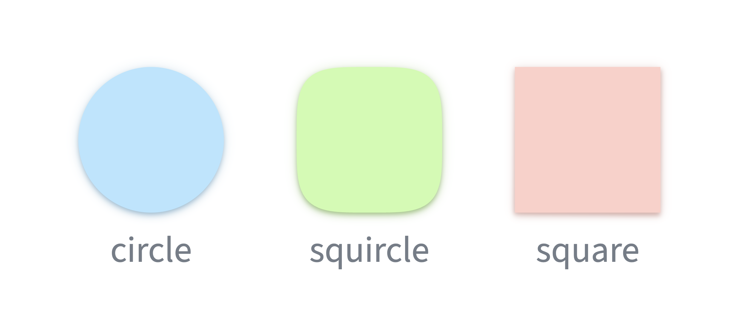
What Are Squircles? And Why Do We Want Them?

A squircle is a geometric shape between a circle and a square; hence the name. Think of it as a rounded square with a unique, pleasant shape. It was first studied in 19th-century mathematics and got popularized in architecture and design. Apple introduced it into the digital world for iOS icons. Nowadays, it is finally supported in browsers. In this article, I discuss how to use squircles in CSS and how to approximate them with cubic Bézier curves, for example, for drawing them into canvas or SVG.

Let's discuss a different shape: a rectangle. We want to avoid sharp corners. Studies in design and user interfaces show that objects with sharp corners are unpleasant. So, let's smooth them out. We see such objects everywhere in the real world.

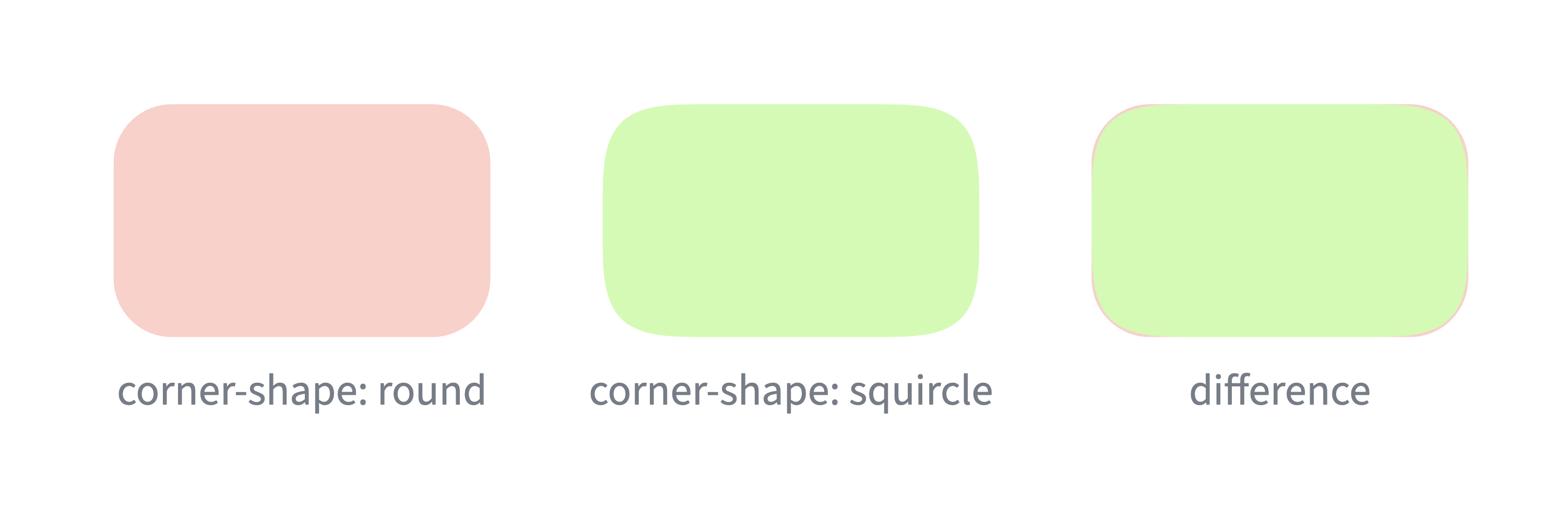
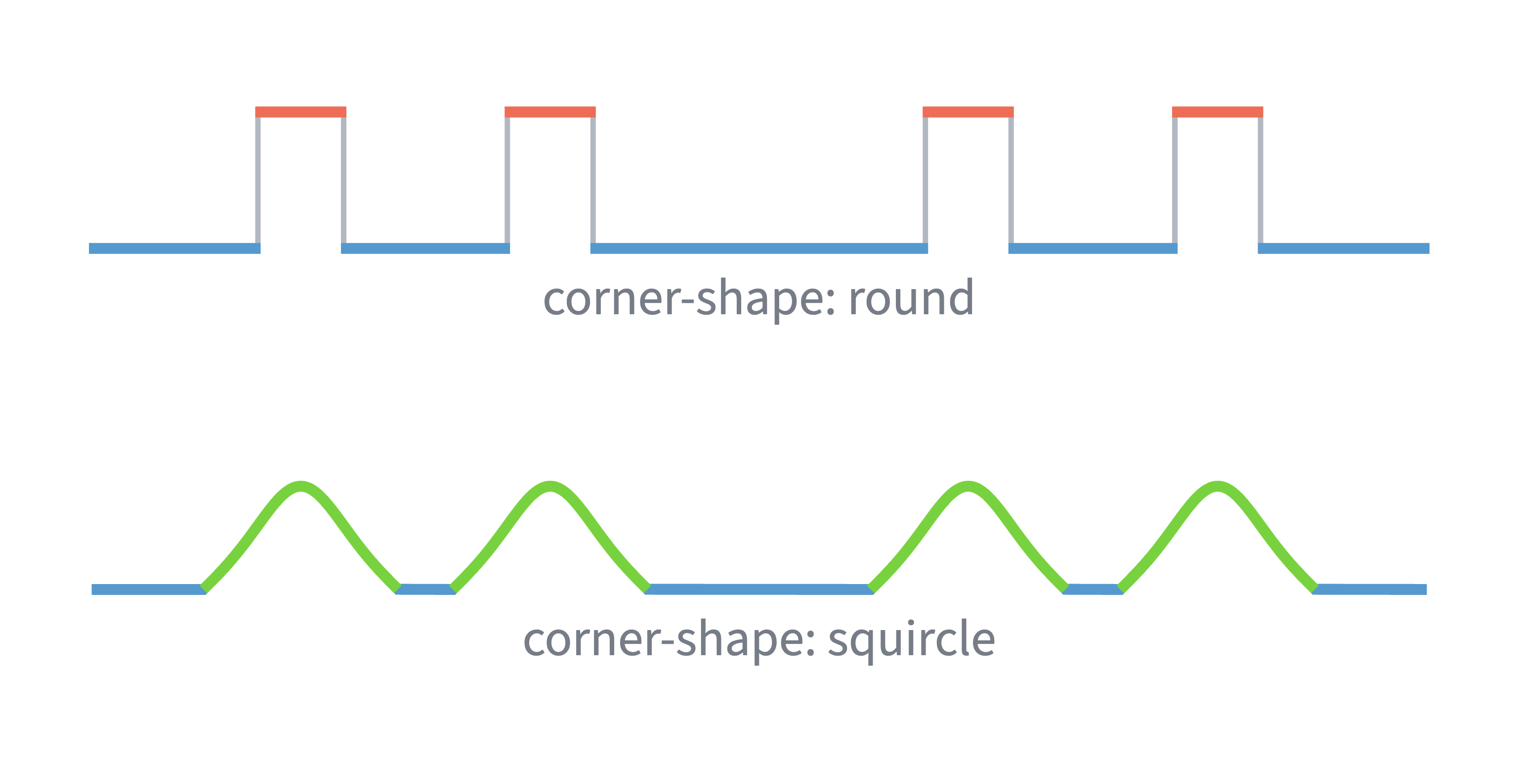
The classical solution is to combine the rectangle with circles. Corners are replaced by tiny quarter circles, whose radius can be chosen. In CSS, this shape is described by the border-radius property. See the red shape below.

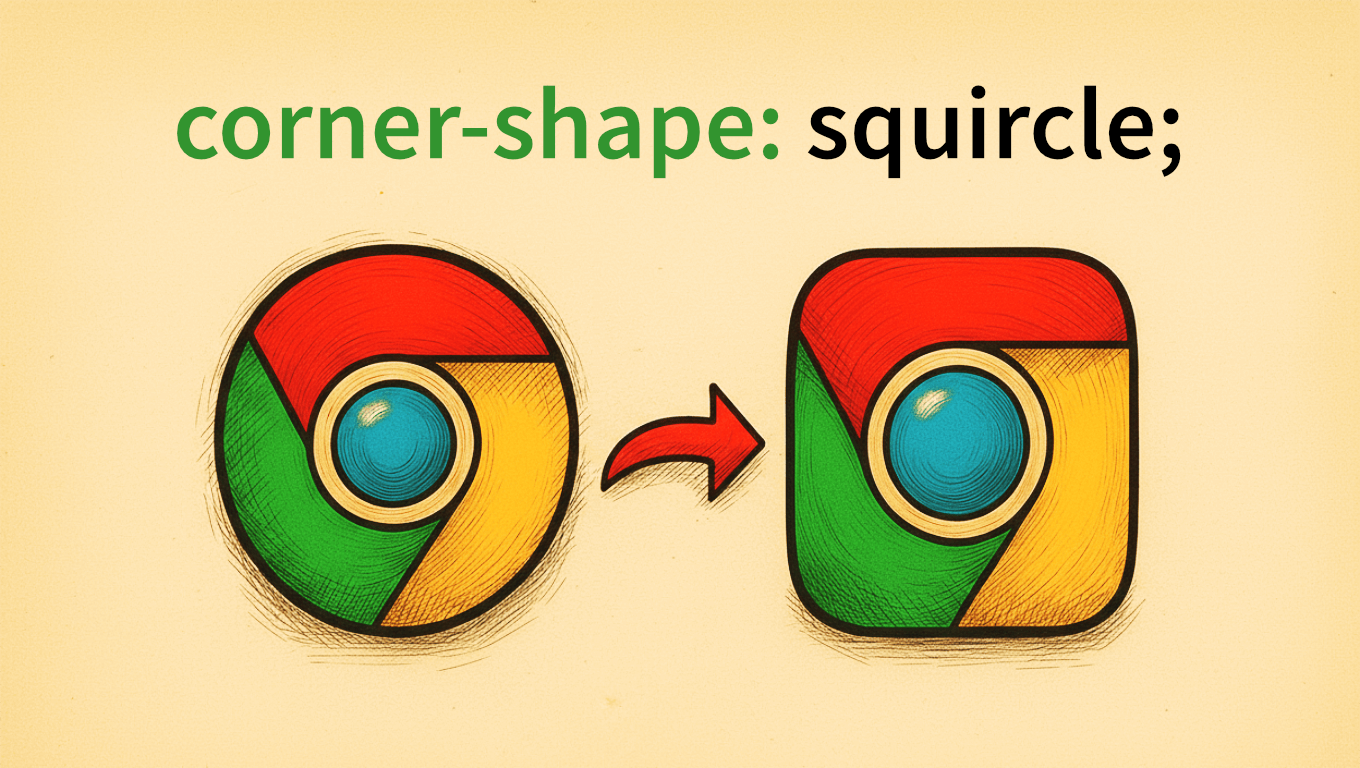
Instead of circular corners, we want to use squircles. To match the overall roundness, we double the radius. This results in the green shape below. The overall look is similar, but the transition from straight to round is more pleasant. In CSS, this can be achieved by a newly introduced corner-shape: squircle property.

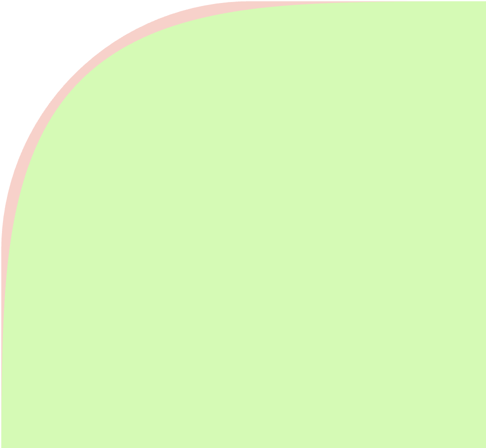
To better see the difference between these shapes, let's zoom into a single corner. The difference seems small, but it is profound!

Problem with classical rounded corners

For seven years, I have been working on the visual environment of the canvas web application OrgPad. My work often blends tech and art, combining programming, math and design. I have learned that human eyes are incredibly sensitive, so even tiny inaccuracies or a single dropped frame don't go unnoticed. And the classical rectangle with circular corners has a hidden flaw. There is something off about the shape, and once you understand it, you will never see it the same.

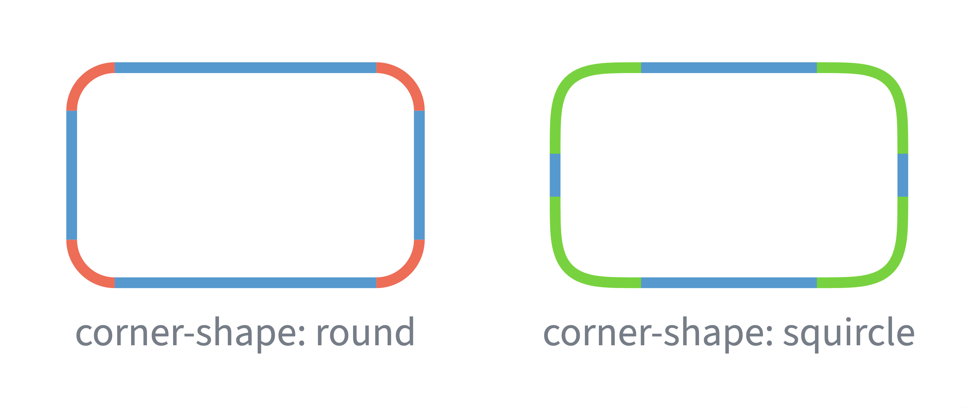
In the picture below, I am comparing circular and squircle corners. On the left, the shape suddenly transitions from straight segments into rounded ones: they don't fit well together. But the squircle transition is gradual and very pleasant. If I didn't use different colors on the right, you wouldn't even notice where one shape starts and the other ends.

In mathematical language, we talk about curvature. The derivative of a function at each point tells how much the function grows/shrinks there. Similarly curvature describes at each point of a curve how much it turns there. Straight segments have curvature equal zero. Circles of radius $\text{[math]}$ have constant curvature $\text{[math]}$ ; so smaller circles turn more sharply than larger ones.

For a rectangle with circular corners, the curvature graph is discontinuous: it jumps between 0 and $\text{[math]}$ . The eye perceives the jump and tries to fix it by imagining a different shape. When we see a circular corner, we instinctively expect the curve to keep turning, which makes it seem as if larger circles are bulging out of the rectangle. With squircle corners, the change in curvature is continuous, so the shape seamlessly transitions from straight to round segments.

Smooth changes in curvature are essential in industrial design. A sudden jump in curvature would be visible in light reflection, making the object very ugly. And when designing roads, we don't want to have sudden turns, instead turning rate should increase gradually. If you are interested in more details, check out this beautiful video by Freya Holmér.

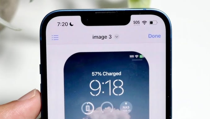
It is no wonder that these ideas were introduced into the digital world by Apple. Their unique position between hardware and software allowed them to see the connections. If you have any Apple device, you can check that the rounded corners are indeed not circles.

Goal of this article

I first learned about squircles a couple years ago and loved the idea. Unfortunately, browser support was poor, so there was no easy way to add them to OrgPad. We rely heavily on HTML rendering, where rounded cells have box shadows. Those shadows visually indicate that there is more content inside. The only option to modify the cell shapes was to use the CSS clip-path property. But this also clipped the shadows.

Everything changed in the summer of 2025, when the new CSS corner-shape property landed in Chrome. Finally, squircles are supported, including box shadows. Adding squircle corners in CSS now requires only a few lines, which I will show in the next chapter. When I saw this change, I knew we can make squircles in OrgPad happen! The entire change took about three days, and you can check it out.

I said that OrgPad uses HTML rendering for cells. But this is no longer true. We have transitioned to rendering most of OrgPad's cells directly with the 2D canvas. It is much faster, and with better control over the rendering quality. For example, the cell above was fully rendered in canvas, including opening/closing animations.

Unfortunately, there is no direct support for squircles in canvas. Luckily, any shape can be described with cubic Bézier curves. Originally, I was hoping to find some existing solution online or get it out of ChatGPT. While these resources were helpful, I eventually had to figure out a cubic Bézier approximation of a squircle on my own. I have decided to write this article so you don't have to.

This approximation is useful far beyond canvas: rendering in SVG, using it in clip-path, or even completely outside of browser, for example, in your game engine or graphical editor. It uses only three cubic Bézier curves per corner, so the full rounded rectangle consists of just 4 straight segments and 12 cubic Bézier curves. And this approximation is pixel-perfect, even at radii of hundreds of pixels.

If this would be the only goal, the article would be very short. I also want to describe the process how I have found this approximation. So we will explaining the math behind squircles. And how to restrict the space of all possible approximations we have to search. Hopefully, it’ll be an educational read, if you ever need to adapt this approach for other shapes.

Using Squircles in CSS

Chrome 139, released on August 5, 2025, added support for the CSS property corner-shape. The support across browsers is still very limited, but other Chromium-based browsers will pick it up soon. Support in Safari (WebKit) will likely take another year. Firefox support is likely years away, but honestly, who cares about it anymore at this point.

This property allows you to change the shape of rounded corners set by border-radius. There are many other use cases, like creating notches, hexagons, octagons, arrows, chat bubbles; see this, this, and this. For us, essential is the value corner-shape: squircle. It replaces circular corners with much nicer squircle ones.

I have tested how to match the visual feeling of rounded corners. I got the best results by doubling border-radius. In all pictures above comparing circular and squircle corners, I have used twice as big border-radius for squircle corners.

Suppose that we want to preserve the same visual look in browsers which support squircles and in browsers which do not yet support it. We can define the border-radius multiplier CSS variable:

:root {
  --brm: 1;
}

@supports (corner-shape: squircle) {
  :root {
    --brm: 2;
  }
}

Then we will use this variable everywhere where we set border-radius. For example, suppose that we have:

border-radius: 16px;

We add squircle corner-shape and include --brm variable:

border-radius: calc(16px * var(--brm));
corner-shape: squircle;

In browsers which support new corner-shape property, squircle will be used and the radius will be multiplied by two. As a fallback, the original border-radius with circle corners will be used. That's it, with a few lines, you can instantly improve look of your website. For example, I have used this to quickly improve look of this website I have built.

There are two issues I have to mention.

There is no problem with circles. They are beautiful shapes with constant curvature. So you probably don't want to use corner-shape: squircle on them, unless you prefer the squircle shape instead.

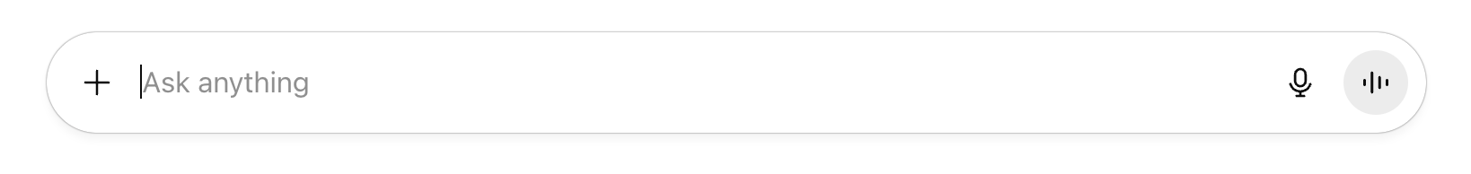
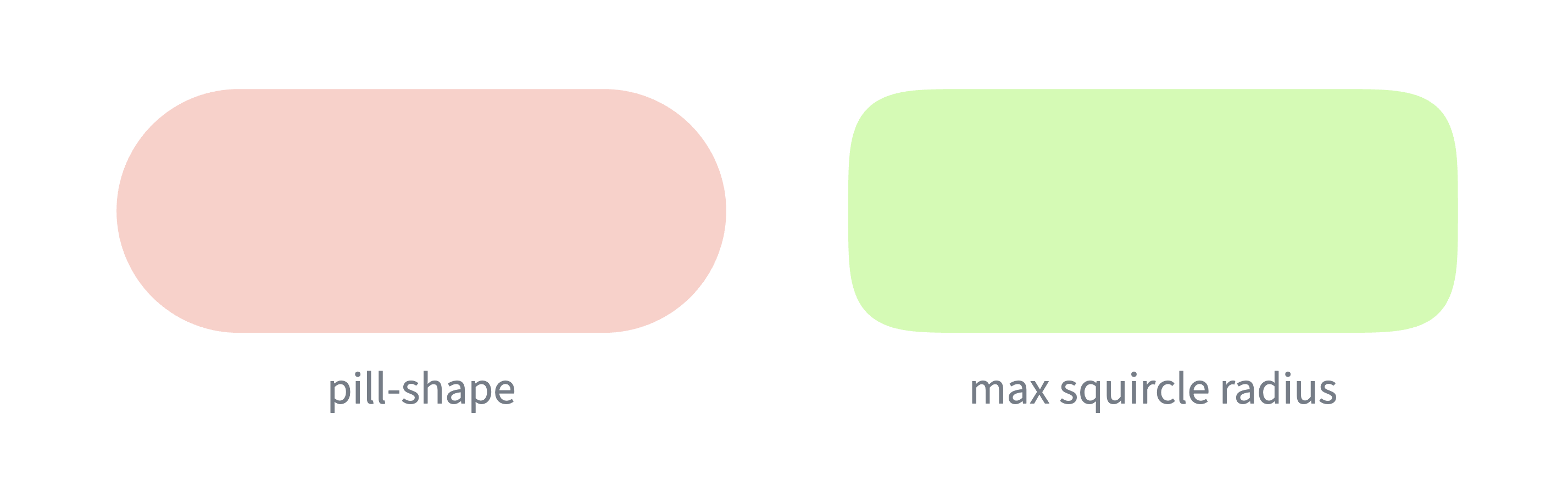
Pill shapes are not possible. These shapes got quite popular in design for buttons and inputs. They have border-radius equal to 50 % of the smaller dimension (usually height). For example, this is the ChatGPT input:

Pill shapes have the same visual problem as rectangles with circular corners since the curvature jumps between the straight and rounded parts of the shape. Once you notice the problem, it is impossible to unsee it.

Unfortunately we cannot fix this with corner-shape: squircle. Since the border-radius has to be multiplied by two, we can only effectively achieve radius of 25 %. So the resulting shape will be much less rounded. We would need a different shape which would smoothly increase and then decrease the curvature. This is not solved by the new corner-shape property. Such a waste!

Mathematics of Squircles

Before looking at the Bézier approximation of a squircle, I want to take a look at the basic math behind it. It will give us a better understanding of what is going on. Luckily, my background is in math and computer science, where I have spent a decade at university doing research and teaching it. You can check my math videos on YouTube.

By working on squircles, I have learned quite a lot new along the way. I have never studied area called differential geometry. One of these days, I will have to check Visual Differential Geometry and Forms by Tristan Needham. His Visual Complex Analysis is one of my favorite math books.

Definition of Squircle

The squircle of radius 1 consists of all points $\text{[math]}$ satisfying the equation

$\text{[math]}$

The equation $\text{[math]}$ gives an arbitrary radius $\text{[math]}$ , but we can easily get the same shape by scaling the squircle of radius 1 by $\text{[math]}$ .

In comparison, the classical circle satisfies the equation $\text{[math]}$ . Higher powers mean the shape is in corners closer to the square.

Circle, squircle, and square belong to the family of shapes called pseudocircles, which are shapes satisfying the equation

$\text{[math]}$

for some parameter $\text{[math]}$ . We get the circle for $\text{[math]}$ , the squircle for $\text{[math]}$ , and the square for $\text{[math]}$ .

Parametric Expression

We want to describe the curve by a parametric expression as the collection of all points $\text{[math]}$ for some functions $\text{[math]}$ and $\text{[math]}$ as $\text{[math]}$ , usually called time, goes from 0 to, say, $\text{[math]}$ . For example, in case of the circle, we get the well-known parametric expression

$\text{[math]}$

The circle curve starts at $\text{[math]}$ and moves counterclockwise.

For the squircle $\text{[math]}$ , let's concentrate, for simplicity, only on the first quadrant, so $\text{[math]}$ . We get the parametric expression

$\text{[math]}$

This solution is found by substituting $\text{[math]}$ and $\text{[math]}$ , which turns the squircle equation $\text{[math]}$ into the circle equation $\text{[math]}$ .

Using Different Coordinates

For our approximation, we just care about the top right corner of the squircle of radius 1. The other three corners can be easily obtained by rotating this approximation. And other radii are constructed by scaling.

We use the standard coordinates in computer graphics, where $\text{[math]}$ is in the top left corner, $\text{[math]}$ grows to the right, and $\text{[math]}$ grows to the bottom. So the entire corner fits within the box from $\text{[math]}$ to $\text{[math]}$ .

The original formulas for $\text{[math]}$ of the squircle start on the right side at $\text{[math]}$ and go around in the counterclockwise direction. We want to start at the top and go in the clockwise direction. So we have to swap the functions for $\text{[math]}$ and $\text{[math]}$ and shift the start towards $\text{[math]}$ . Therefore, the top right corner of the squircle consists of all points $\text{[math]}$ where

$\text{[math]}$

These points can be computed by the following Clojure code:

(defn squircle-point
  "Computes the point of the squircle at the given time for radius 1, centered at [0 1].
  For t=0, the curve starts at [0 0] and moves in the clockwise direction."
  [t]
  [(math/sqrt (math/sin t))
   (- 1 (math/sqrt (math/cos t)))])

Derivatives and Tangent Directions

For some time $\text{[math]}$ , we also want to know the slope of a tangent line at the point $\text{[math]}$ . This slope is $\text{[math]}$ , where $\text{[math]}$ and $\text{[math]}$ are derivatives of the parameter:

$\text{[math]}$

We can compute these derivatives with the following Clojure code:

(defn squircle-derivative
  "Computes the vector of derivatives of the squircle at the given time. The squircle
  is centered at [0 1] and has radius 1. For t=0, the curve starts at [0 0]
  and moves in the clockwise direction."
  [t]
  (let [c (math/cos t)
        s (math/sin t)]
    [(* 0.5 c (/ (math/sqrt s)))
     (* 0.5 s (/ (math/sqrt c)))]))

Curvature

Curvature of a curve determines at each point how much it is turning there. So, the straight line has curvature zero everywhere, and a circle of radius $\text{[math]}$ has the constant curvature $\text{[math]}$ .

The curvature $\text{[math]}$ at the point $\text{[math]}$ is determined by the radius $\text{[math]}$ of the best possible touching circle approximation at this point. We have $\text{[math]}$ . The formula for $\text{[math]}$ consists of first- and second-order derivatives of $\text{[math]}$ and $\text{[math]}$ :

$\text{[math]}$

Let's compute the curvature of the squircle. We have already seen the first-order derivatives. The second-order derivatives are as follows:

$\text{[math]}$

By plugging these into the curvature formula, everything nicely simplifies into

$\text{[math]}$

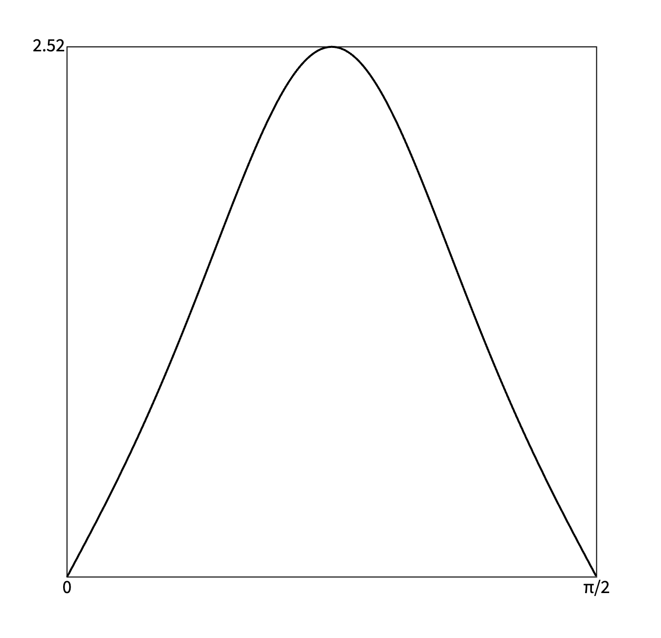
The graph of curvature of the squircle looks like this:

So the curvature starts at zero, continuously grows, peaks at $\text{[math]}$ and then symmetrically decreases back to zero. This allows the squircle corner to be smoothly glued with a straight segment.

This Clojure code computes second-order derivatives and curvature of the squircle:

(defn squircle-second-derivative
  "Computes the vector of second derivatives of the squircle at the given time.
  The squircle is centered at [0 1] and has radius 1. For t=0, the curve starts
  at [0 0] and moves in the clockwise direction."
  [t]
  (let [c (math/cos t)
        s (math/sin t)]
    [(+ (* -0.5 (math/sqrt s))
        (* -0.25 (math/pow s -1.5) (* c c)))
     (+ (* 0.5 (math/sqrt c))
        (* 0.25 (math/pow c -1.5) (* s s)))]))

(defn squircle-curvature
  "Computes unsigned curvature of the squircle at the given time.
  The squircle is centered at [0 1] and has radius 1. For t=0,
  the curve starts at [0 0] and moves in the clockwise direction."
  [t]
  (let [c (math/cos t)
        s (math/sin t)]
    (/ (* 3 s c)
       (math/pow (+ (* s s s) (* c c c)) 1.5))))

Finding Cubic Bézier Approximation

Since the 2D canvas does not have built-in squircles, we want to describe them using cubic Bézier curves. This won't be exact; it just needs to be accurate enough for our needs. And to make it fast, we want to use as few Bézier curves as possible. A good approximation by Bézier curves is useful in other situations, for example in SVG, in CSS clip-path, and even completely outside the browser. And I have found a great one that is extremely accurate and uses just three cubic Bézier curves per corner.

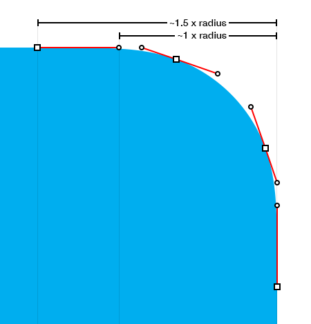
My starting point was this blog post about squircles by Figma. People tried to reverse engineer Apple iOS app icons, and found out that they construct each corner by three cubic Bézier curves. This image was very helpful. Unfortunately, iOS app icon is not based on a squircle but a pseudocircle for $\text{[math]}$ , so we can't use these cubic Bézier curves directly.

Cubic Bézier Curves

Each cubic Bézier curve $\text{[math]}$ , where $\text{[math]}$ goes from 0 to 1, is described by four arbitrary points in the plane:

two endpoints $\text{[math]}$ and $\text{[math]}$ ,
two control points $\text{[math]}$ and $\text{[math]}$ .

The formula for the curve is

$\text{[math]}$

This animation from Wikipedia shows how the curve evolves as $\text{[math]}$ goes from 0 to 1.

For our purpose, the behavior right after 0 and right before 1 matters.

Right after 0, the curve heads almost linearly from $\text{[math]}$ to $\text{[math]}$ as $\text{[math]}$ , since $\text{[math]}$ is almost one and both $\text{[math]}$ and $\text{[math]}$ are negligible. Of course, as $\text{[math]}$ grows, the influence of both $\text{[math]}$ and $\text{[math]}$ grows.
The situation is reversed when $\text{[math]}$ is almost 1. The curve moves almost linearly in the direction from $\text{[math]}$ to $\text{[math]}$ , and the impact of $\text{[math]}$ and $\text{[math]}$ is negligible.

How the Approximation Looks

We want to approximate the top right corner of the squircle with just three cubic Bézier curves. These three Bézier curves have four endpoints $\text{[math]}$ , where the first one goes $\text{[math]}$ , the second $\text{[math]}$ , and the last $\text{[math]}$ . Since the corner goes from $\text{[math]}$ to $\text{[math]}$ , we know that $\text{[math]}$ and $\text{[math]}$ . There are further six control points $\text{[math]}$ , two for each Bézier curve.

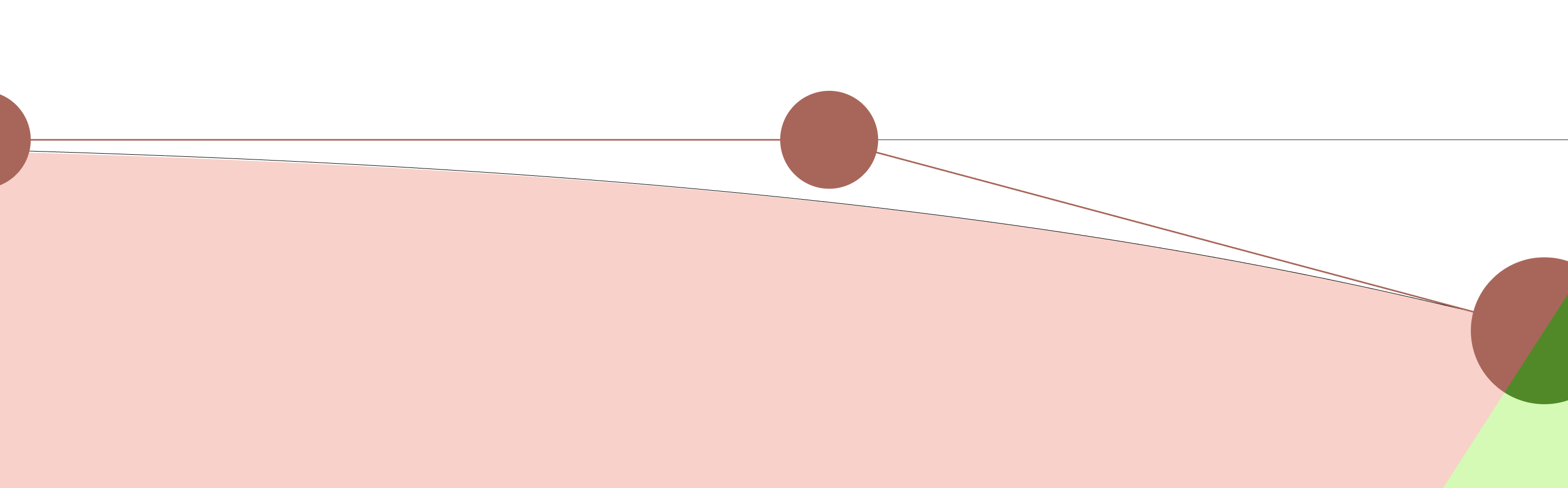
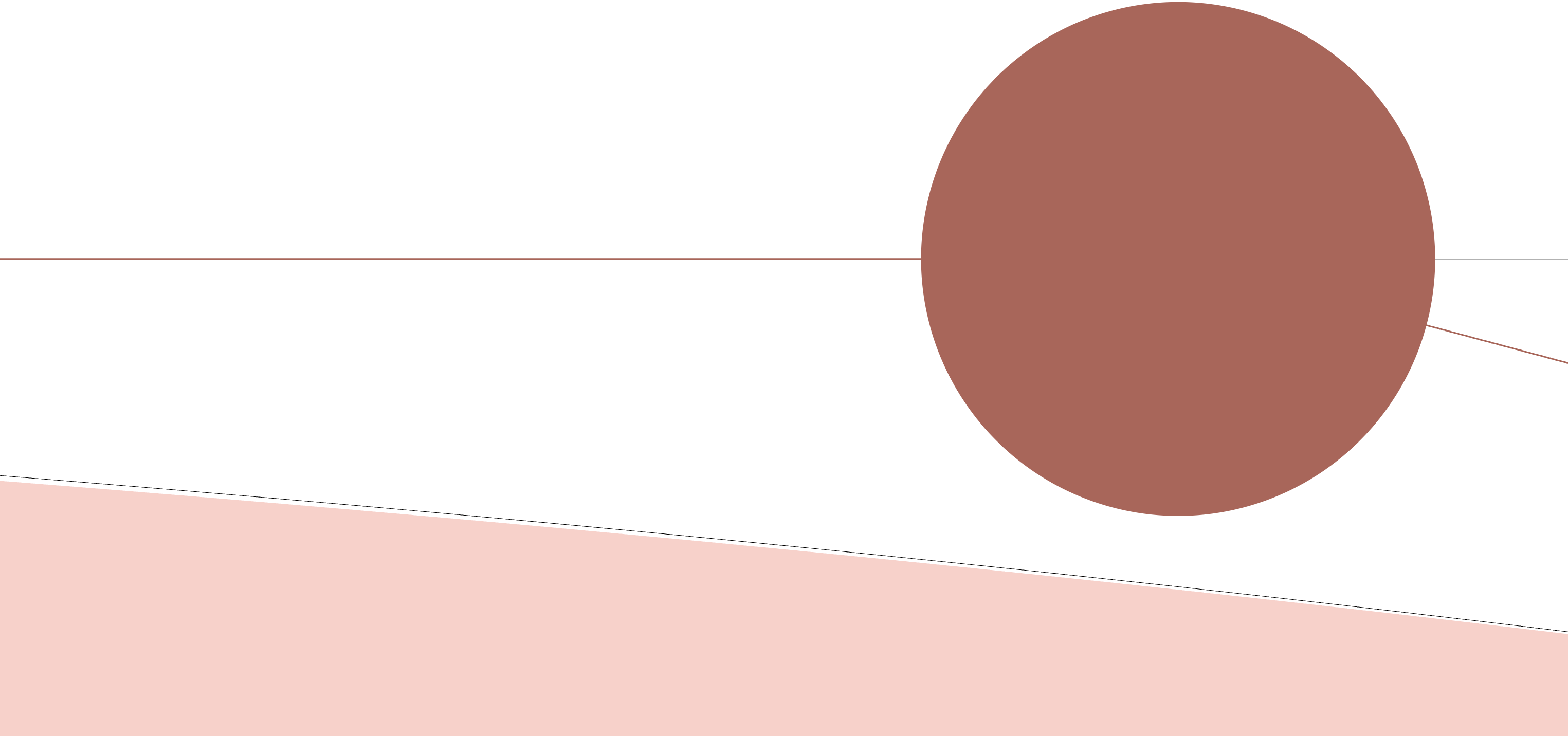
The image below shows the situation. The squircle itself is drawn by a thin black line, constructed by computing $\text{[math]}$ for many points. The three cubic Bézier curves are shown in red, green, and blue: both their larger endpoints and smaller control points. The region bounded by these curves is filled by red, green, and blue.

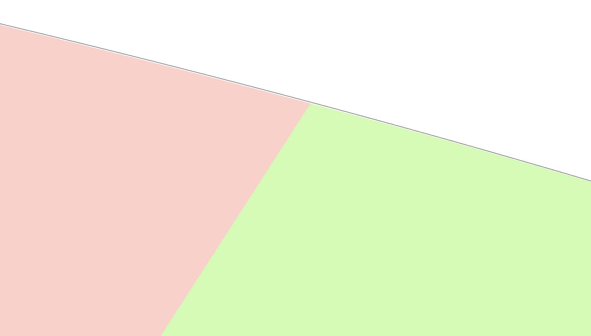
When looking at the image, the filled region seems identical with the precise squircle in black. My approximation is this good! If we zoom in a lot, we will see small errors: either there will be a small white gap in between the black line and the filled region, or the filled region will go slightly behind the black line. If you are interested, check the zoomed in images at the end.

Aside from the added notation, the image above was not created for the purpose of this article. I have built it directly inside OrgPad and have used it while finding my approximation. Whenever one tackles a visual problem, using the right visualization makes things so much easier. When placed directly into OrgPad's canvas, one may nicely move around and zoom in to see the errors in great detail.

Furthermore, we use hot code reloading in OrgPad, so any changes in the code are immediately displayed without having to reload the page. Right after building this visualization, I have quickly noticed some silly mistakes in my coordinates, and the entire process of finding the right constants for the approximation took less than 2 hours.

Finding the Approximation

So let's find positions of all endpoints and control points. Certain relations will be forced, others can be chosen freely. There will be three parameters which can be chosen. I have always used my interactive visualization to find values which make a good fit.

Symmetry of Approximation.

Any reasonable approximation has to be symmetric by the diagonal axis $\text{[math]}$ , since the squircle corner is symmetric by this axis. So $\text{[math]}$ , $\text{[math]}$ , $\text{[math]}$ , $\text{[math]}$ , and $\text{[math]}$ . So we just need to determine the position of $\text{[math]}$ This restricts the number of choices we have to do by half.

Choice #1: Position of $\text{[math]}$ .

Since $\text{[math]}$ lies somewhere on the squircle, its position is determined by choosing some time $\text{[math]}$ . I have tried a few options and ended up right in the middle with $\text{[math]}$ . It is certainly possible to build great approximations with other choices of $\text{[math]}$ .

In this way, the first and last Bézier curves approximate each quarter of the time interval $\text{[math]}$ , while the middle one approximates the remaining half. Visually, the squircle changes more slowly when around $\text{[math]}$ , so using the middle curve for a longer interval is no problem.

$\text{[math]}$ , $\text{[math]}$ , and $\text{[math]}$ are collinear.

Another restriction comes from the fact that we glue these three Bézier curves together. We certainly don't want to have sharp hinges' where the direction of the approximation sharply changes when it enters, say, $\text{[math]}$ . In the language of control points, this means both $\text{[math]}$ and $\text{[math]}$ lie on a line passing through $\text{[math]}$ . So we just need to choose some slope and both $\text{[math]}$ and $\text{[math]}$ are determined by two distances from $\text{[math]}$ on this slope.

Tangent slope at $\text{[math]}$ .

What is this slope? Recall that when $\text{[math]}$ is right around $\text{[math]}$ , the direction towards the nearest control point has the strongest influence. So the Bézier curve moves almost linearly towards this control point. Therefore, locally, the best possible slope is the tangent direction of the squircle at point $\text{[math]}$ , which is $\text{[math]}$ . For $\text{[math]}$ , we get the following approximate slope when rounded to three digits:

$\text{[math]}$

Both $\text{[math]}$ and $\text{[math]}$ lie on this slope passing through $\text{[math]}$ . We just need to determine their distances. These distances can be chosen independently, since one distance determines the approximation before $\text{[math]}$ and another one after $\text{[math]}$ .

Choice #2: Position of $\text{[math]}$ .

Since I was constructing the approximation visually inside OrgPad, I just zoomed in a lot into the green region and tried various values for this distance. This was super easy, since my visualization automatically updated as I changed the constants in my code. In my code, I specified the distance as a multiple of the distance between $\text{[math]}$ and $\text{[math]}$ . I found that the multiplier 0.395 works really well.

Position of $\text{[math]}$ .

The goal of our Bézier approximation is to match the curvature of the squircle as closely as possible. Ideally, the initial and final curvatures should be exactly zero. As observed in this Figma article, this is achieved by placing $\text{[math]}$ on the same line. So both $\text{[math]}$ and $\text{[math]}$ have to lie on the top line.

On the other hand, we have already placed $\text{[math]}$ somewhere on the tangent line at $\text{[math]}$ . Therefore, the position of $\text{[math]}$ is uniquely determined by their intersection.

Choice #3: Position of $\text{[math]}$ .

We want to place $\text{[math]}$ somewhere on the top line between $\text{[math]}$ and $\text{[math]}$ , and we are free to choose this position $\text{[math]}$ Again, I zoomed in a lot and tried different values. I got a really good approximation for $\text{[math]}$ .

Putting It Together

To generate the list of endpoints and control points for each of three Bézier curves, I have written the following Clojure function:

(defn compute-squircle-bezier-approximation
  "Computes endpoints and control points for three cubic Bézier curves, approximating
  the top-right squircle corner of radius 1, see squircle-bezier-approximation below.
  The first curve starts at A=[0 0], the last one ends at D=[1 1]. These Bézier
  curves are also symmetrical along the axis going between [1 0] and [0 1].

  The computation is determined by three parameters:

  - t is the time of the first middle target point B on the squircle. The other
    point C is computed by the reflection.
  - a determines the position of the first control point C1 = [a 0]. The second
    control point also lies on the top line, so the initial curvature is zero,
    matching the straight segment.
  - m is the multiplier for the distance of B and C which gives the distance
    of C2 and B."
  [t a m]
  (let [axis [[0 1] [1 0]]
        A [0 0]
        B (squircle-point t)
        C (reflect-by-line B axis)
        D [1 1]
        tangent-dir (normalize (squircle-derivative t))
        C1 [a 0]
        C1' (:point (lines-intersection-times [A [1 0]] [B (vec- B tangent-dir)]))
        C2 (vec+ B (vec* tangent-dir (* m (dist C B))))
        C2' (reflect-by-line C2 axis)
        C3 (reflect-by-line C1' axis)
        C3' (reflect-by-line C1 axis)]
    [[A C1 C1' B]
     [B C2 C2' C]
     [D C3 C3' D]]))

During development, I changed the input parameters and ended up with the values we just derived:

(compute-squircle-bezier-approximation (/ math/pi 8) 0.3 0.395)

Cubic Bézier Approximation of a Squircle

The top-right corner of a squircle of radius 1, going from [0,0] to [1,1], can be approximated by three cubic Bézier curves: each determined by two endpoints and two control points in the middle. They have the following positions when rounded to three digits:

Start point	Control point 1	Control point 2	End point
[0, 0]	[0.3, 0]	[0.473, 0]	[0.619, 0.039]
[0.619, 0.039]	[0.804, 0.088]	[0.912, 0.196]	[0.961, 0.381]
[0.961, 0.381]	[1, 0.527]	[1, 0.7]	[1, 1]

The other three corners can be easily constructed by rotating these curves, and different radii are achieved by scaling the approximation. Overall, each rectangle with squircle corners can be drawn using 4 straight segments and 12 cubic Bézier curves. So, it is really fast!

Here is Clojure code which renders a rectangle with corners rounded according to the squircle curve. In squircle-bezier-approximation data, I am only storing two control points and the endpoint for each curve, since I only need these in ctx.bezierCurveTo. The previous endpoint is reused.

(def squircle-bezier-approximation
  "Bézier control points and target points for three cubic Bézier segments
  forming top-right corner of a squircle with radius 1, starting
  at [0 0] and ending at [1 1]. This approximation is similar to iOS squircle
  icon approximation."
  [[[0.3 0] [0.473 0] [0.619 0.039]]
   [[0.804 0.088] [0.912 0.196] [0.961 0.381]]
   [[1 0.527] [1 0.7] [1 1]]])

(defn squircle-corner!
  "Draws a single squircle corner at the given start position, radius, and rot-multiplier
  of 90 degrees."
  [^js ctx start radius rot-multiple]
  (when (pos? radius)
    (doseq [[cA cB target] squircle-bezier-approximation
            :let [cA' (vec+ start (vec* (rot-by-90 cA rot-multiple) radius))
                  cB' (vec+ start (vec* (rot-by-90 cB rot-multiple) radius))
                  target' (vec+ start (vec* (rot-by-90 target rot-multiple) radius))]]
      (cubic-curve-to! ctx cA' cB' target'))))

(defn squircle-rect!
  "Draws the rectangle with squircle corner shape, the given top-left
  and bottom-right corners and corner radius. We assume that radii
  together are less than each of the sides. It is possible to supply
  different radii for all four corners."
  ([^js ctx [left top :as top-left] [right bottom :as bottom-right] radius]
   (squircle-rect! ctx top-left bottom-right radius radius radius radius))
  ([^js ctx [left top] [right bottom]
    radius-top-left radius-top-right radius-bottom-right radius-bottom-left]
   (let [start-top-right [(- right radius-top-right) top]
         start-bottom-right [right (- bottom radius-bottom-right)]
         start-bottom-left [(+ left radius-bottom-left) bottom]
         start-top-left [left (+ top radius-top-left)]]
     (doto ctx
       (move-to! [(+ left radius-top-left) top])
       (line-to! start-top-right)
       (squircle-corner! start-top-right radius-top-right 0)
       (line-to! start-bottom-right)
       (squircle-corner! start-bottom-right radius-bottom-right 3)
       (line-to! start-bottom-left)
       (squircle-corner! start-bottom-left radius-bottom-left 2)
       (line-to! start-top-left)
       (squircle-corner! start-top-left radius-top-left 1)
       (close-path!)))))

If you are not familiar with ClojureScript, here is the equivalent code in JS, generated by ChatGPT. It is also available as a CodePen.

// Bézier control points for the top-right squircle corner (radius = 1)
const squircleBezierApproximation = [
  [[0.3, 0],       [0.473, 0],     [0.619, 0.039]],
  [[0.804, 0.088], [0.912, 0.196], [0.961, 0.381]],
  [[1, 0.527],     [1, 0.7],       [1, 1]]
];

const vecAdd = ([x1, y1], [x2, y2]) => [x1 + x2, y1 + y2];
const vecMul = ([x, y], k) => [x * k, y * k];

// Rotate 90° clockwise * k
function rotBy90([x, y], k) {
  switch (k % 4) {
    case 0: return [x, y];
    case 1: return [y, -x];
    case 2: return [-x, -y];
    case 3: return [-y, x];
  }
}

// Draw a single squircle corner
function squircleCorner(ctx, start, radius, rotMultiple) {
  if (radius <= 0) return;

  for (const [cA, cB, target] of squircleBezierApproximation) {
    const cA2 = vecAdd(start, vecMul(rotBy90(cA, rotMultiple), radius));
    const cB2 = vecAdd(start, vecMul(rotBy90(cB, rotMultiple), radius));
    const t2  = vecAdd(start, vecMul(rotBy90(target, rotMultiple), radius));

    ctx.bezierCurveTo(cA2[0], cA2[1], cB2[0], cB2[1], t2[0], t2[1]);
  }
}

// Draw squircle rectangle (single or four radii)
function squircleRect(ctx, topLeft, bottomRight, rTL, rTR, rBR, rBL) {
  const [left, top] = topLeft;
  const [right, bottom] = bottomRight;

  if (rTR === undefined) {
    rTR = rBR = rBL = rTL;
  }

  const startTR = [right - rTR, top];
  const startBR = [right, bottom - rBR];
  const startBL = [left + rBL, bottom];
  const startTL = [left, top + rTL];

  ctx.moveTo(left + rTL, top);
  ctx.lineTo(startTR[0], startTR[1]);
  squircleCorner(ctx, startTR, rTR, 0);
  ctx.lineTo(startBR[0], startBR[1]);
  squircleCorner(ctx, startBR, rBR, 3);
  ctx.lineTo(startBL[0], startBL[1]);
  squircleCorner(ctx, startBL, rBL, 2);
  ctx.lineTo(startTL[0], startTL[1]);
  squircleCorner(ctx, startTL, rTL, 1);
  ctx.closePath();
}

The squircleRect function is then used like this:

const canvas = document.querySelector('canvas');
const ctx = canvas.getContext('2d');

ctx.beginPath();
squircleRect(ctx, [20, 20], [280, 180], 28); // uniform radius
ctx.fill();

ctx.beginPath();
squircleRect(ctx, [320, 20], [580, 180], 12, 36, 24, 48); // four radii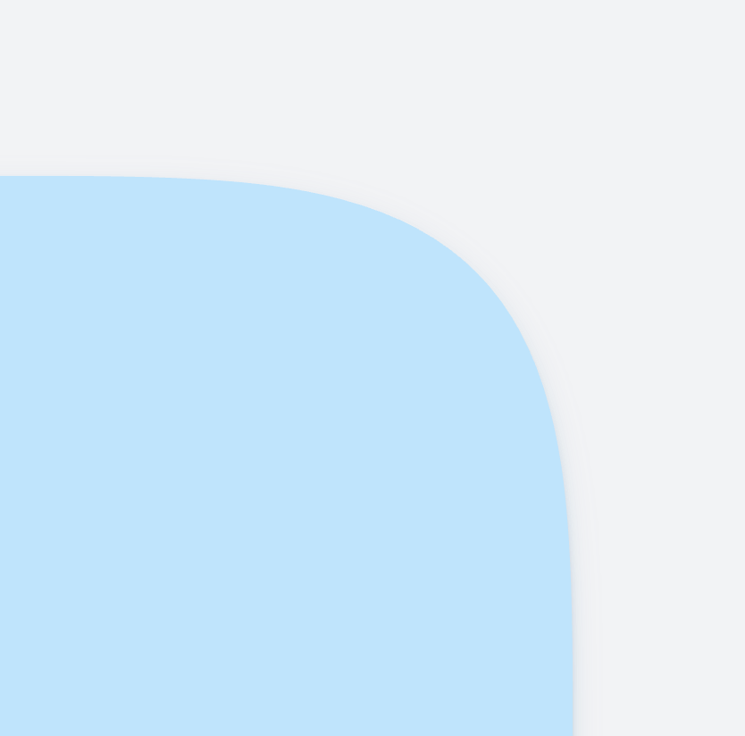
ctx.stroke();

Is This the Best Approximation?

Surely not! But I didn't pursue it any further. The accuracy is already much, much higher than anything I need in OrgPad. And OrgPad's requirements are huge compared to most websites. In OrgPad, the maximum supported zoom is 5×. When fully zoomed in, the largest possible visible border radius is 340 px (680 px on Retina displays). Below, you can see one corner of a cell, fully zoomed in on a Retina display. At this scale, the approximation is still pixel-perfect.

To find the real optimum, one could explore the full space of three parameters. For that, we would need to define the error function and then find its minimum for all possible choices. If you find a better approximation, please let me know so I can update this article.

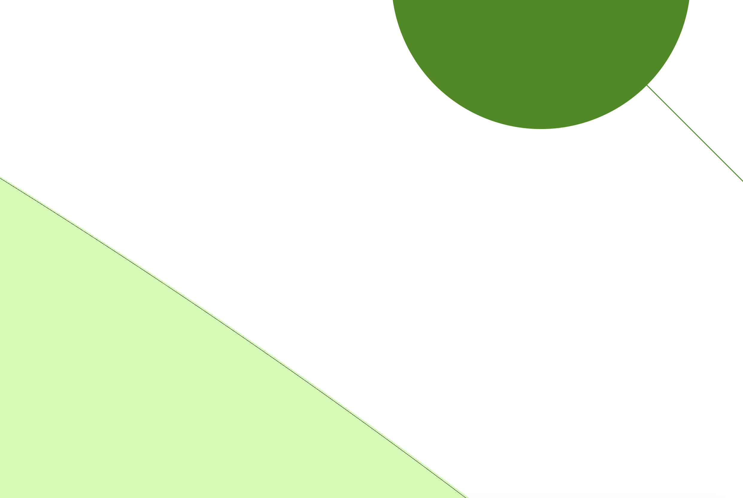
So how good is the approximation? It is really good. It will be completely perfect even when the radius is of hundreds pixels. In 10× zoom, we still do not see any errors in our visualization. In 100× zoom, the errors finally become visible. If you really care about this level of accuracy, using some adaptive Bézier approximation will be necessary. But for all practical purposes in graphics, this accuracy is sufficient.

Curvature of the Approximation

Let's also visualize curvature of these Bézier curves. The approximation consists of three different parts with tiny discontinuity in the middle. It fits really nicely.

These Bézier curves join with tiny discontinuities in curvature. But the difference is so small that it is not visible. You can check it for yourself below where I have removed the Bézier endpoints and control points.