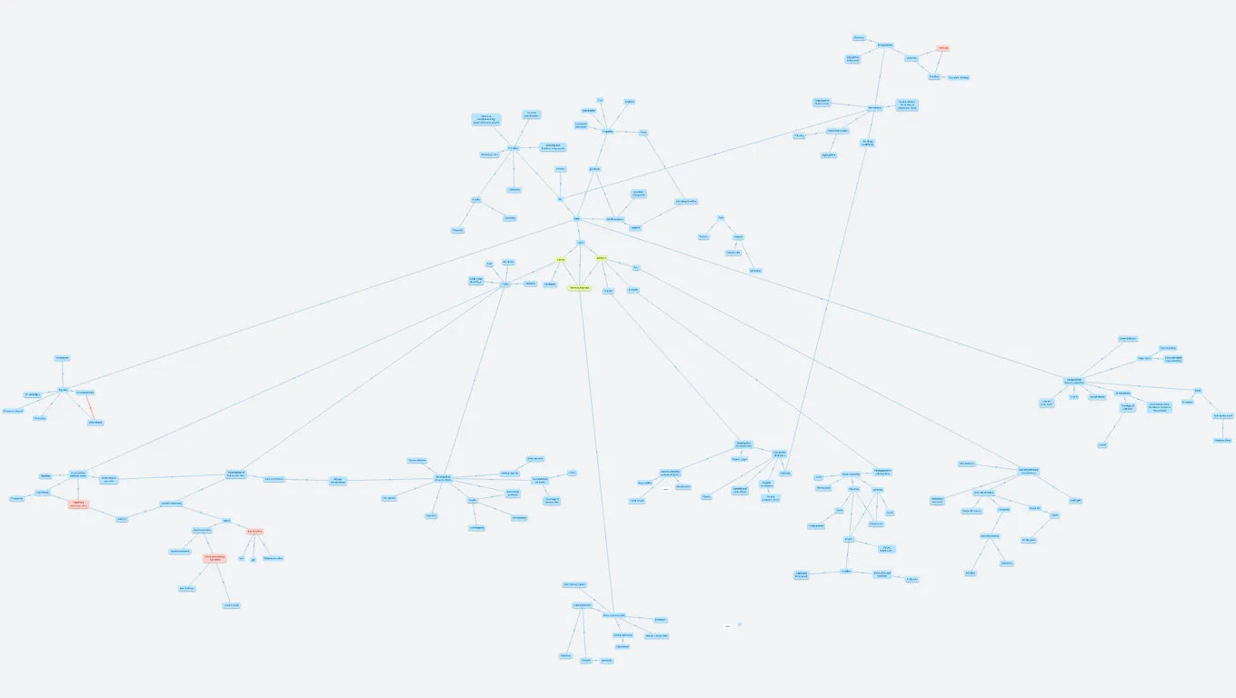
VIZ

Created by Michal Mikeska

Visualization of vector fields

Texture based methods

Zooming

Geometric

Semantic

Fisheye

Manipulation

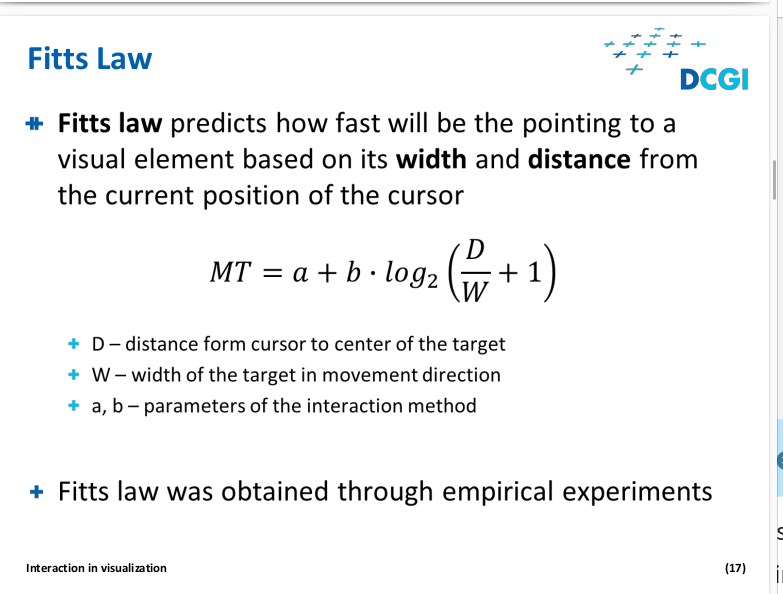
Fitts law

Navigation in the data

Overview and detail - spatial separation

Pan and zoom - temporal separation

Focus + context - deformation

Selection

• Values of attributes
• Pointing
• Fitts law
• Improved pointing
• Brushing

Pointing

Voronoi pointing

Bubble

Excentric labeling

Size

Position

Organization of data views

• Juxtaposition, Superimposition,
• Embedding Linked/coordinated views
• Multiform/multiple views
• Shared encoding views
• Brushing and linking

Shneiderman’s Taxonomy of Interaction Tasks

Overview

Filer

Zoom

Details on Demand

Relate

History

Extract

Accuracy, discriminability, separibility and popout

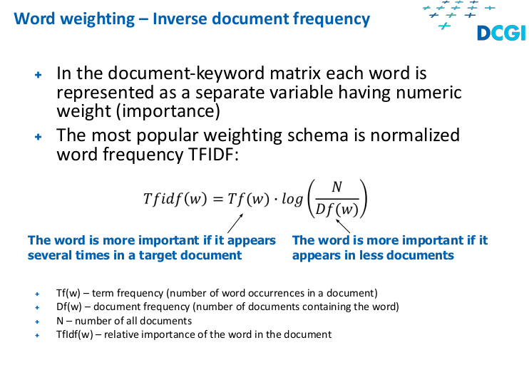
The number of different values that need to be shown for the attribute being encoded must not be greater than the number of steps available for the visual channel used to encode it.

Do not use RGB

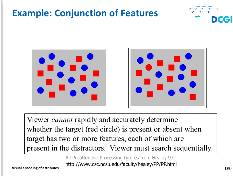
Pop out… visible first

Pop out (preattentive)

Orientation

Interaction

Low level

Higher level

Curvature and shape

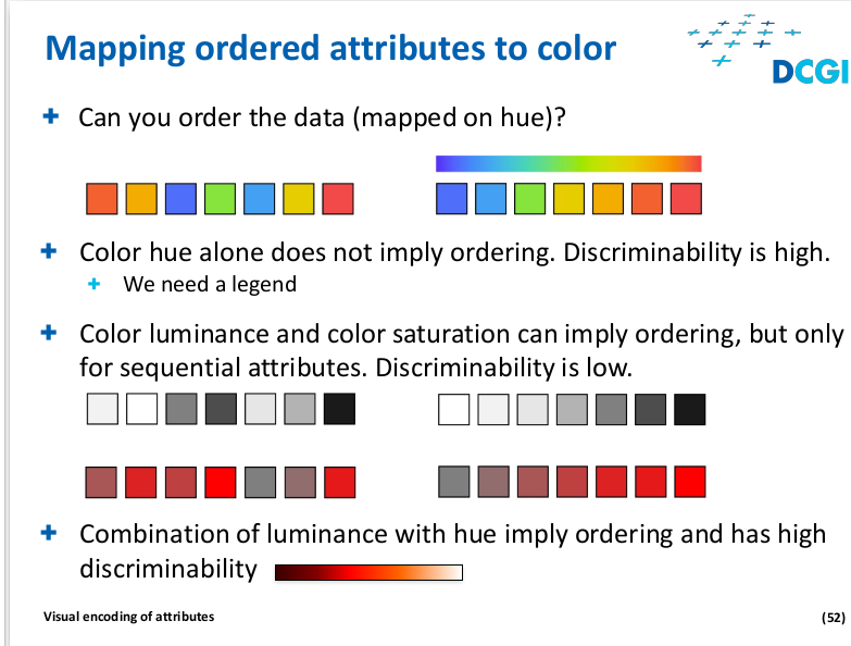
Mapping

Color

3 channels

Luminance, Saturation, Hue

Filtering

Dynamic quereis - classic min max e.g.

Reduction of data

Filering and aggregation

Encoding rules

Expressiveness principle: Visual encoding should express all of, and only, the information in the dataset attributes.

Effectiveness principle: Encode most important attributes with highest ranked channels

Encoding

Absolute and Relative Judgements

Aligned vs Unaligned

Brushing and linking

Aggregation

Binning

Clustering

Statistics distribution

Process

Data

Data enrichment

Filtering

Mapping

Rendering

Attribute

Tufte Rule

Visual attribute value should be directly proportional to data attribute value

Marks

Marks – geometric primitives

• Points
• Lines
• Areas

Viz

Nominal / Categorical

• No inherent order (in the sense of certain quantity)
• People, Companies, Cities, Types of diseases, ...

Ordering direction

• Sequential - the values of the attribute range from minimum to maximumvalue
• E.g., mountain height measured from sea level
• Diverging - the values of the attribute can be split into two groups thatdiverge in positive and negative direction from a common zero point
• E.g., Full elevation dataset containing mountain heights and depths of oceanfloor is diverging
• Cyclic - the values of the attribute wrap around to the starting point
• E.g., Hour of the day, Day of the week

Grouping

Similarity

Connectedness

Containment

Data

Attribute types

Task

Channels

+ Visual channels – control appearance of marks

• Position
• Color
• Tilt
• Size
• Shape

Ordered

Ordinal

• Ordered, but not at measurable intervals
• XS, S, M, L, XL, XXL, XXXL
• Mon, Tue, Wed, Thu …

Quantitative

• Ordered, arithmetic operations are possible
• Discrete: Integers
• Continuous: Floats

Types

Actions

Analyze

• Consume: Discover,Present, Enjoy
• Produce: Annotate,Record, Derive

Query (dotaz)

• Identify
• Compare
• Overview/Summarize

Search

• Lookup, Locate
• Browse, Explore

Targets

• All data - Trends, Outliners, Features
• Atrributes - one vs many

Spatial data

shape

Distance / proximity

Grid

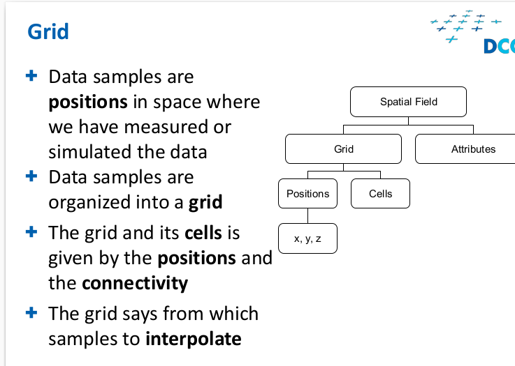
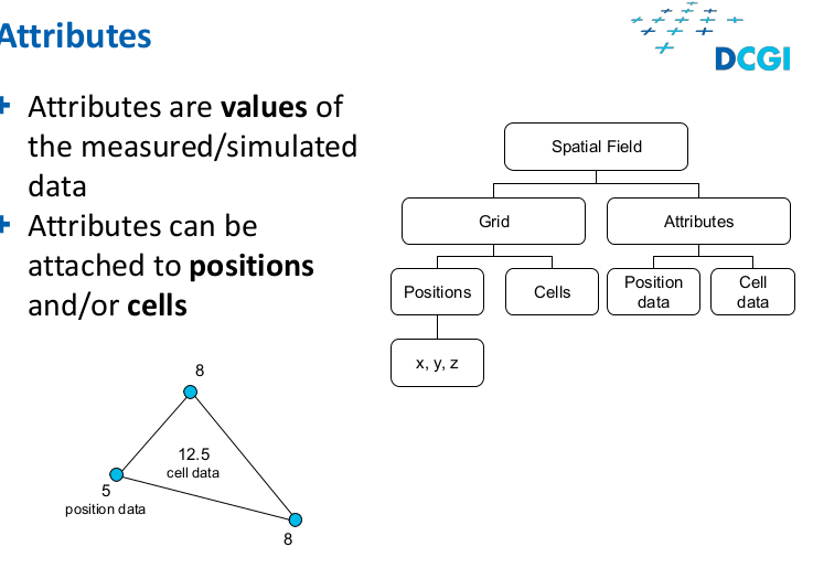
Attribute

Spatial

Abstract

Text

Document

• Sections
• Words

Collection of documents

• Source code

Networks

Underlying field F(x,y)

F - dependent / it s attribute

x,y - independent

Fields

• Grids
  • Positions
  • Cells
• Attributes

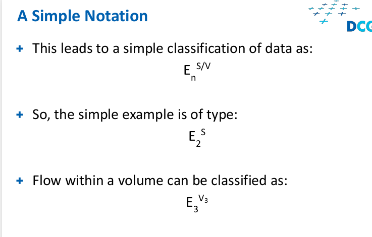
Notation

Geometry

• Meshes
  • Vertices
  • Edges
  • Faces
  • Typically, no attributes

Time varying data

Attributes and/or their

structure (topology) change

in time

Tabular

Tables

• Items
• Attributes

Relation

Networks

• Items
• Links
• Attributes

Data attributes

Cartograms, glyphs

Edge bundling

Techniques

Regresion

Box plots

Confidence interval

Signature-based detection

Outlier/Intrusion Detection

Anomaly Detection

Trajectories

Force-directed edge bundling

Geographical data visualization

3V- definition

3V-definition: Big data is high-volume, -velocity and -variety

information assets that demand cost-effective, innovative forms of

information processing for enhanced insight and decision making.

Big data

Visual analytics

How do i treat data?

If we have quantitative attribute measured at geographic locations, we treat the data as scattered spatial data

If we have nominal attribute obtained at geographic locations, we cannot treat the data as spatial filed

Layers

Raster model

Change the real data into grid

Area, midpoint, importance

Vector model

Maps

Topological relations

Arc - node model

Acceleration Data Structures forVector Data Model

Mercator

Frequency-based

Clustering

Data mining

Visual Data Mining

• New approach for exploring very large data sets
• Combination of traditional mining methods and visualization techniques+Advantages
• Combination of strengths of data mining and visualization+Challenges
• User needs to select the appropriate data mining technique in a givensituation
• Find visualization techniques suitable for the results of data miningoperations
• User needs to be experienced both in data mining and in visualization

Label placement

Usable label layout should exhibit 4 main characteristics +

• Readability – we can read all labels
• Unambiguity – we can associate label with the labeled feature
• Compactness – the map is not larger because of the labels
• Aesthetics – the label layout should look nice (aesthetics are subjective)

Visualization of tabular data

Model

Topology Connectivity: Arcs are connected to others (at nodes). This identifies possible routes and networks, such as rivers and roads, via the lists of arcs and nodes in the database.

• Containment: An enclosed polygon has a measurable area;lists of arcs define boundaries and closed areas.
• Contiguity: The adjacency of polygons can be determinedby shared arcs.
• These are fundamental to GIS analysis and queries, forexample:+
• From point A, how can I get to point B using the city road system?
• What is the area of the combined areas of all residential housing?
• Which residential areas are next to city parks?

Objcects, lines

Stream ribbons

Colormap vorticity

Euler method

x(t+dt) = x(t) + v(x(t))·dt

Shape / glyps

Continuous attributes

Text analysis

Lexical

Syntactic

Semantic

Mapping

Grayscale, blind ppl., intuitive

Visualization of scalar fields

Color

Should be HCL

Discrite,nominal, ordinal attributes

Faceting

Scatterplot matrix

Brushing

Visualization of relation data

Text and software visualization

Types of grids and cells

regular,uniform, rectiliner,curvilinear

Visualisation of Volumetric data

Volumetric data are spatial fields

• 3D scalar field

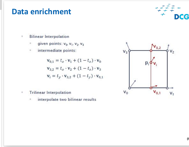
Data enrichment

• Nearest neighbor
  • Value in every point of space correspond to the value of the nearest sample
• Linear interpolation
• Cubic interpolation

Stream objects

Some flow

Bilinear interpolation

Aggregation

Good

Connections

Proximity

Visual encoding

Properties

• The tangent to a contour line is the direction of the height field’s minimal (zero) variation
• The perpendicular to a contour line is the direction ofthe height field’s maximum variation: the gradient

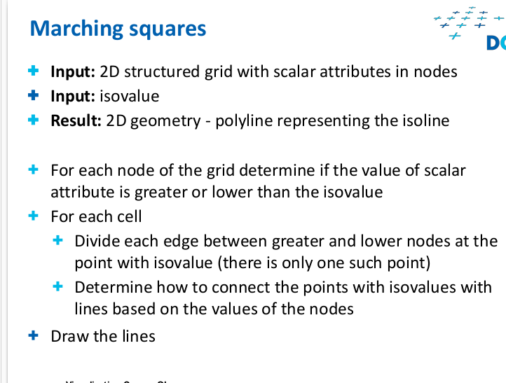
Contouring

A contour line C is defined as all points p in a dataset D that have the same scalar value, or isovalue s(p)=x

Perceptual problems

No interpolation

Sparse vs scalar field is dense

amples

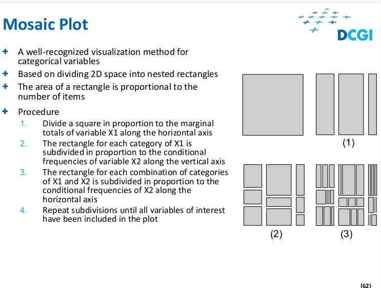
Mosaic plot

Glyphs

Star glyphs

Chernoff faces

Stick figures

Binning

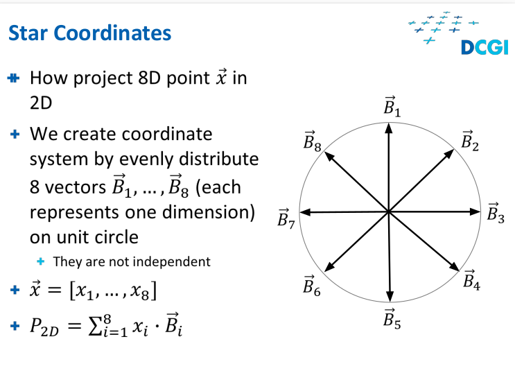
Dimensional projections

Star projection - maybe no clusters

Parallel coordinates

Not so good

Similarity

Containment

Hiearchy

Network

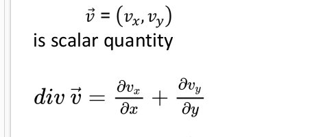
Divergence

Sink is minus

Plus is source

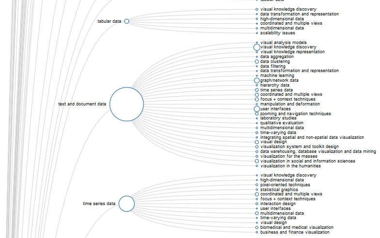
Text visualization

Document

Corpus

Streams

Marching squares / cubes

Volume rendering

Indirect

• Intermediate geometric representation
  • Cutting plane, tiny cubes, iso-surface
• Pros: Easy shading, perception of shape, fast rendering – can bedivided into conversion to geometry and rendering
• Cons: Occlusion, no context

Direct

• No intermediate geometric representation
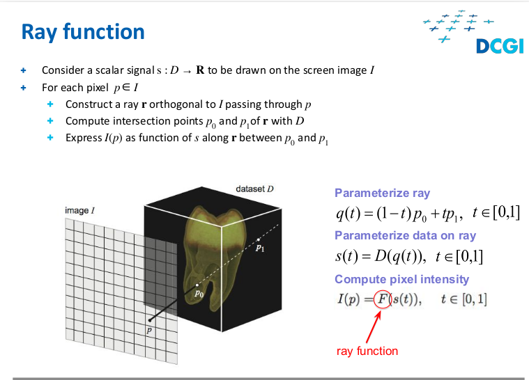
  • Ray function, Ray integration
• Pros: Illustrate the interior, semi-transparency, great flexibility
• Cons: High computational cost, large memory requirements

Glyphs

Just arrow or line, it s mapping technique of vector fields

Line integral convolution

• Correlate with neighboring texture values along theflow (in flow direction)
• Do Not correlate with neighboring texture values across theflow (normal to flow direction)

Parallel sets

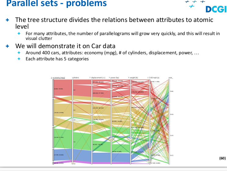
Trends, outliners, focus

Document metadata

Software

Relation data

Diagrams

See soft

Indirect

2d planes

Tiny cubes

Countouring - iso surface calculation

Vorticity

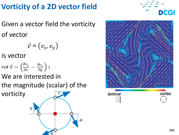
cross product give us the orientation of the rotation

Good

Containment

Connections

Good

Connections

Containment not scalable!

Single document

Word Cloud

Facet clouds

Spark clouds

TempoTaggram

Collection

Linguistic

Direct

Resampling

Random vs uniform

Better for rotated

Types

Word Tree

Netspeak WordGraph

DocuBurst

Phrase Nets

Ray integration

Mapování na barvu a průhlednost pomocí transfer funkce

Overlapping

Glyph longer then distance between samples..sometimes not problem

We can take every second sample...subsampling

Containment

Using tree map

Cannot use!

Similarity

Proximity

Ray function

Graphs

Doc-term matrix

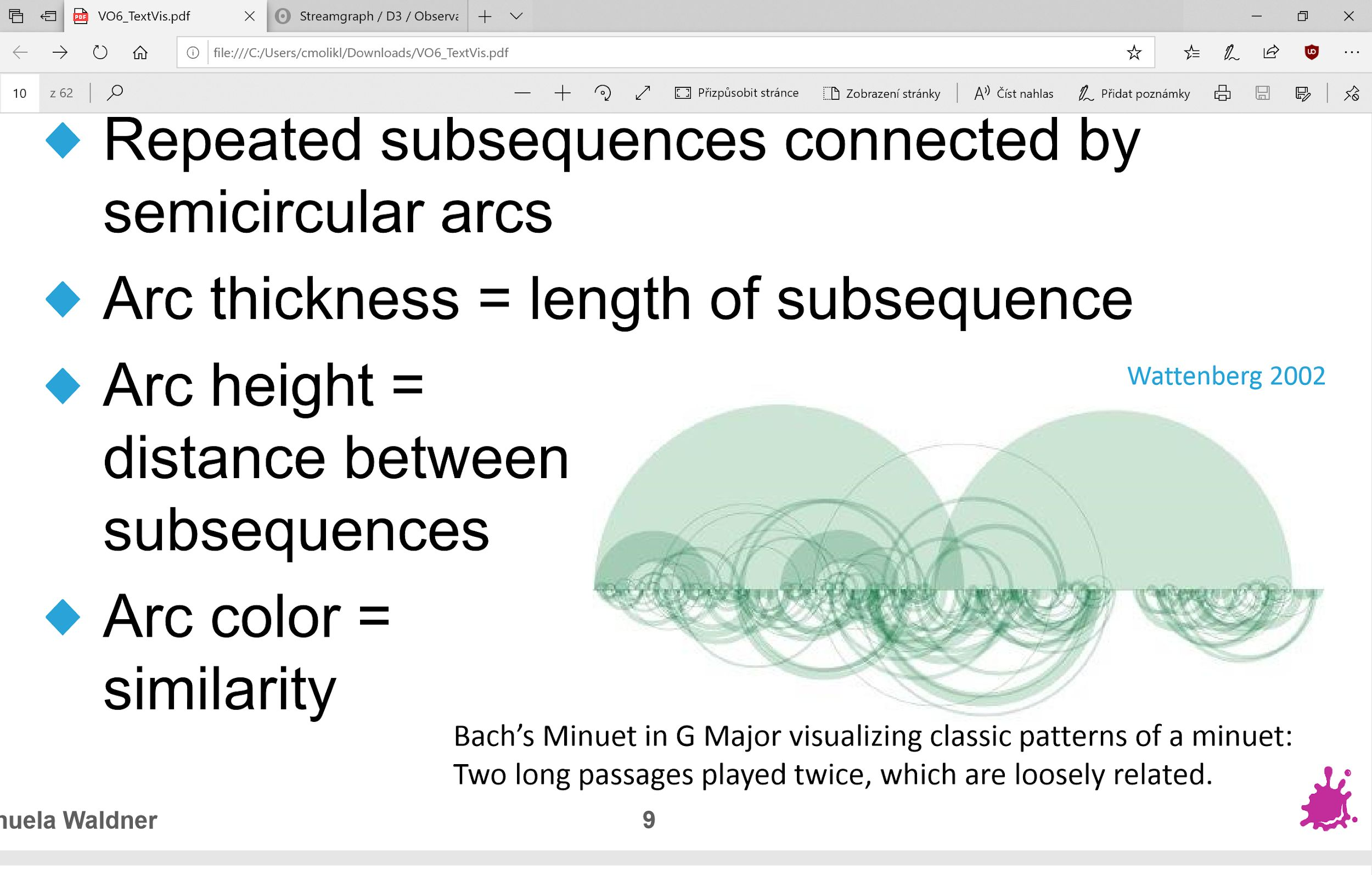
Arcdiagram

Transfer function

1D - 1 attribute

2D - 2 attribute

To color and opacity

Ballon, radial, cone...

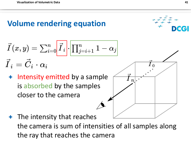
Volume rendering equation

MIP

AIP

Distance to value

Similarity

cosine product

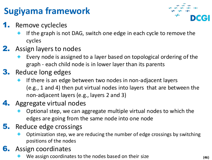
Sugiyama framework

Creation

Force-directed methods

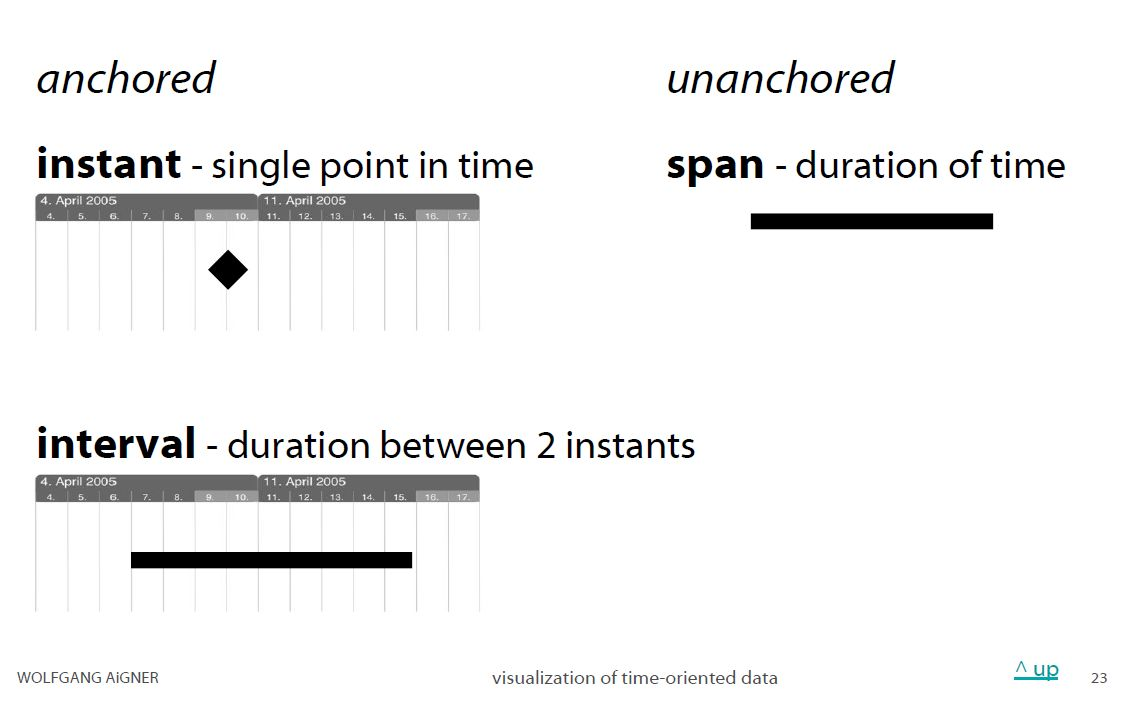
Intervals and spans

Ganchart

Net trees

Problems

• They do not consider edge crossings
• Hairball result for densegraphs
• The result is very oftena local minimum

Weights

Back to front

• We need to calculate only one equation in each sample

ba

Front to back

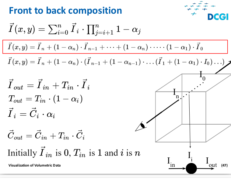
• We need to calculate two equations for each sample
• When the opacity reaches a defined “large” value the process ends we terminatethe composition

Time primitives

Time-oriented data

Examples

Spiral graphs

Faceting

Cycle plots

Text Insight via Automated Responsive Analytics (Tiara)

amples

Granularity issue

Instans spatial data

Lexis pencil

Helix icons

GeoTime

Conversion

Relations

E.g. google calendar

Domain

Ordinal

Discrete

Continuous

structure

Linear

Cyclic

Branching